
building a bigger qwen out of two qwen models
a crash course in model chimerism

tl;dr: Take a giant Qwen3 MoE model, collapse its experts into a dense stack that matches Qwen3-8B’s width, then interleave those dense MoE blocks with the 8B blocks to create a deeper hybrid. Validate that the transplanted blocks actually matter, fix the ‘hot’ ones, and end with a model that’s both larger and reasonably sane.
Why does this work at all?
Qwen3-8B and Qwen3-235B-A22 share the same hidden size and attention head dimension. If hidden size matches, you can line up linear layers across both networks without inventing sketchy adapters. The other knobs still matter (kv-heads, RoPE, tokenizer, layernorm flavor), but those are tractable.
The end result here is a 64-layer dense model with Qwen3-8B widths. Rough parameter math helps orient the scale:
Per block, LLaMA/Qwen‑style attention + MLP is about 3hi + 4h² parameters with h = 4096 and i = 12288, which is ≈ 218.1M each.
Tied embedding/lm_head adds V · h once; with V ≈ 152k, that’s ≈ 0.623B.
So, a model with L layers has about 0.623 + 0.218 × L billion parameters. With L = 64, you land near 14.6B.
The plan
The process has three phases: collapse the MoE, interleave to build depth, then prove and tune influence.
Phase 1: collapsing the MoE to dense
MoE layers aren’t directly usable inside a dense stack, so the first step is to turn each expert bundle into a single FFN that looks like the base. The key steps are:
Average the experts per projection (don’t concatenate them1).
Fix FFN orientation: up and gate are [intermediate, hidden], down is [hidden, intermediate]. PyTorch stores weights as [out, in].
Remap attention heads correctly under GQA.
q has out = num_heads · head_dim
k and v have out = num_kv_heads · head_dim
o has in = hidden
When the source and target differ in kv-heads, group-average or repeat heads, then adjust head_dim by truncate/pad as needed.
# collapse -> dense to 8b dims (averaging experts)

proj$ python moe_to_dense.py \
  --model_id Qwen/Qwen3-235B-A22B-Instruct-2507 \
  --target_model Qwen/Qwen3-8B \
  --output_path ./qwen3-235b-dense-avg \
  --method average \
  --low_memory
Phase 2: interleaving to build a deeper hybrid
Now make a deeper model by sampling a subset of collapsed MoE blocks and splicing them between base blocks across the depth. The simplest plan aims for evenly distributed insertions and keeps the base config and tokenizer. RoPE stays the base’s RoPE.
One issue: Qwen3-8B has 36 transformer blocks in the release used here, not 32. So if the final stack is 64, the “even” plan distributes 28 MoE-dense blocks across 64 positions by ratio. It is not clean odd/even parity.
# interleave to 64 layers, even distribution
proj$ python moe_to_dense.py \
--compose_interleaved \
--base_model Qwen/Qwen3-8B \
--moe_converted ./qwen3-235b-dense-avg \
--composite_output_path ./qwen3-8b-plus-moe-64L \
--final_layers 64 \
--interleave_strategy even \
--cast_dtype bfloat16 \
--low_memory
# validate shapes and loading again
proj$ python moe_to_dense.py --validate_model ./qwen3-8b-plus-moe-64L
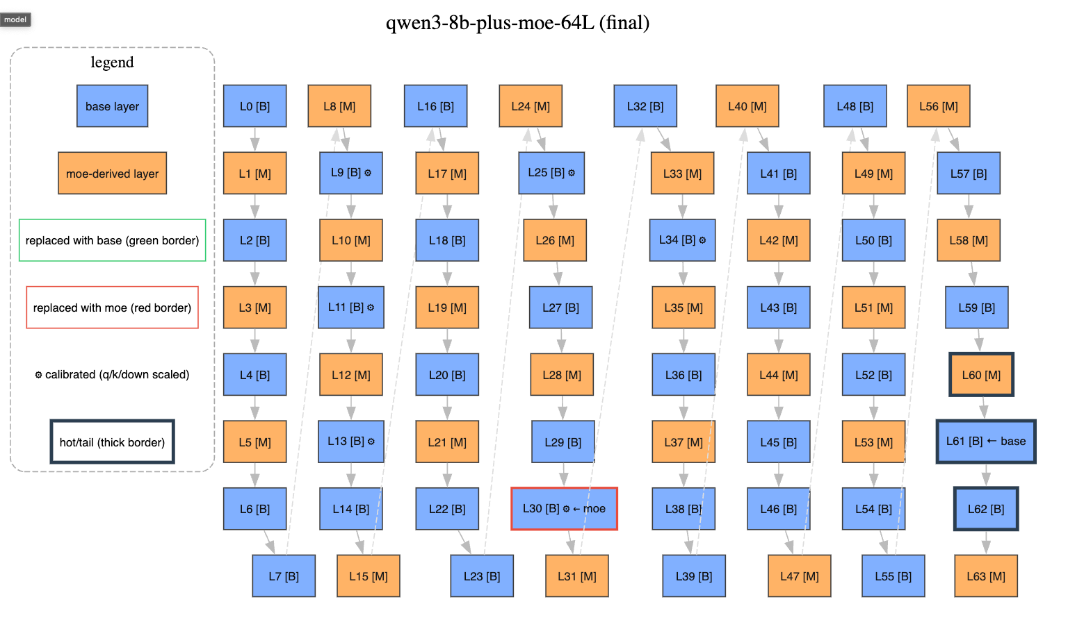
# model loads successfully on meta deviceIn the built stack, the MoE‑derived indices in 0..63 end up something like:
moe: 1, 3, 5, 8, 10, 12, 15, 17, 19, 21, 24, 26, 28, 31, 33, 35,
     37, 40, 42, 44, 47, 49, 51, 53, 56, 58, 60, 63

base: everything else
Phase 3: prove influence and tune it
A hybrid only matters if the transplanted blocks actually move the loss. There are two friendly probes for that: gate scan and swap scan. Both are cheap and run on CPU+GPU with device_map.
Gate scan temporarily zeroes the residual contribution of a layer and records the delta in NLL/perplexity. If turning off a layer barely changes the loss, it’s inert on that dataset. If it hurts a lot, it’s pulling weight.
Swap scan temporarily replaces a composite layer with the mapped base layer and records the delta. If swapping gets worse, the composite layer is doing something different and useful. If it improves, consider swapping permanently.
# gate scan on the tail to find the heavy hitters

proj$ python layer_influence.py \
  --model ./qwen3-8b-plus-moe-64L \
  --layers 48-63 \
  --prompts_file sample.txt \
  --dtype bfloat16 \
  --gate_scan

baseline: ppl ~58.0

top influence when gated off: 62, 60, 53, 55, 48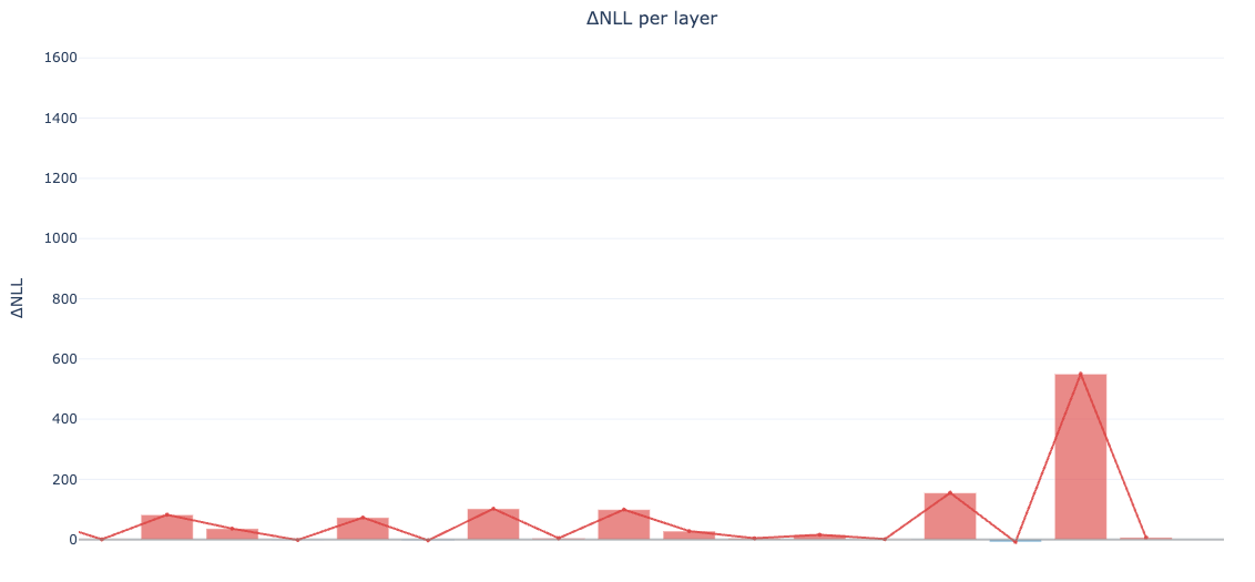
# swap scan with ratio mapping (36 -> 64), same region

proj$ python layer_influence.py \
  --model ./qwen3-8b-plus-moe-64L \
  --donor_model Qwen/Qwen3-8B \
  --layers 48-63 \
  --prompts_file sample.txt \
  --dtype bfloat16 \
  --swap_scan \
  --swap_map ratio

layer 61: swapping to base improves loss a lot

layers 60, 62: swapping to base gets worse
That’s enough info to do a tiny surgery.
Surgery 1: replace a weak block
Layer 61 looked weak. Replacing it with the mapped base block improved baseline perplexity immediately. This is a pure shard edit; no GPU memory needed.
# replace L61 with mapped base and write a new dir

proj$ python layer_surgery.py \
  --composite ./qwen3-8b-plus-moe-64L \
  --base Qwen/Qwen3-8B \
  --out ./qwen3-8b-plus-moe-64L-surgery \
  --replace_layers 61 \
  --map ratio

# recheck gate/swap

proj$ python layer_influence.py \
  --model ./qwen3-8b-plus-moe-64L-surgery \
  --layers 48-63 \
  --prompts_file sample.txt \
  --dtype bfloat16 \
  --gate_scan

baseline: ppl ~48.0

tail still strong: 62, 60, 55, 53
The last block is its own animal. Swapping layer 63 with the base one caused an insane meltdown, which is expected. Do not swap it. Just leave 63 alone.
Surgery 2: damp ‘hot’ attention and FFN
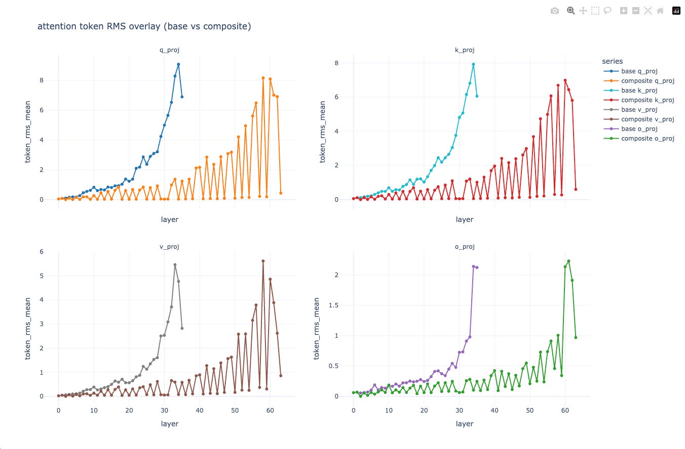
Now that the tail is healthy, look across the whole stack for pockets that push in the wrong direction. The activation stats script helps visualize where attention or MLP spikes appear.
# collect activations and write a stats json

proj$ python activation_stats.py \
  --model ./qwen3-8b-plus-moe-64L-surgery \
  --prompts_file sample.txt \
  --dtype bfloat16 \
  --tensorboard_dir runs/act_stats \
  --save_json stats.json \
  --attention_entropy

# visualize with a small dashboard

proj$ python visualize_activations.py \
  --stats_json stats.json \
  --out_html stats.html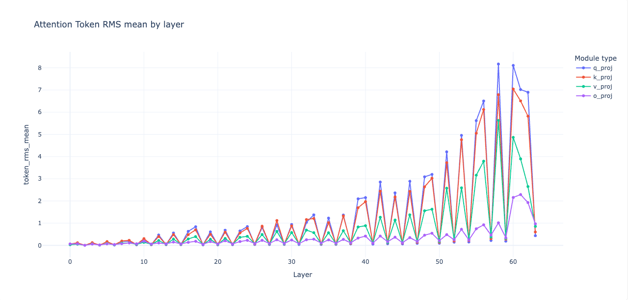
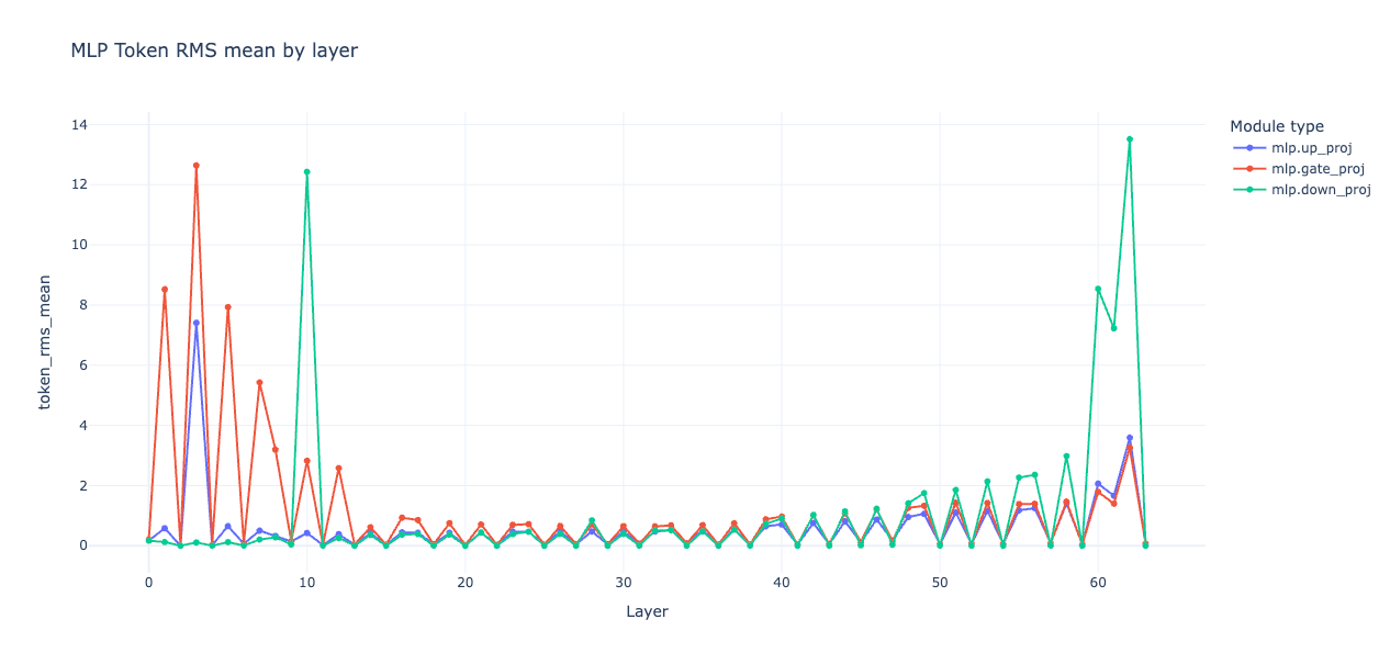
A passable heuristic is to gently shrink q and k on layers where attention alone reduces loss when gated, and to shrink mlp.down on layers where MLP alone reduces loss. These are scalar multipliers on the relevant weight matrices. A little goes a long way.
# scale a handful of layers by a few percent

proj$ cat scales.json
{
  "9":  { "attn_q": 0.96, "attn_k": 0.96, "mlp_down": 0.98 },
  "11": { "attn_q": 0.90, "attn_k": 0.90 },
  "13": { "attn_q": 0.90, "attn_k": 0.90 },
  "25": { "attn_q": 0.92, "attn_k": 0.92 },
  "30": { "attn_q": 0.88, "attn_k": 0.88, "mlp_down": 0.95 },
  "34": { "attn_q": 0.90, "attn_k": 0.90 }
}

proj$ python layer_surgery.py \
  --composite ./qwen3-8b-plus-moe-64L-surgery \
  --out ./qwen3-8b-plus-moe-64L-surgery-cal \
  --scale_json scales.json

# confirm deltas got small and baseline moved the right way

proj$ python layer_influence.py \
  --model ./qwen3-8b-plus-moe-64L-surgery-cal \
  --layers 9,11,13,25,30,34 \
  --prompts_file sample.txt \
  --dtype bfloat16 \
  --gate_scan

baseline: ppl ~47.8

deltas: small negatives only (≈ −1 to −7), mostly attention
Surgery 3: one block swap mid‑stack
One mid-stack base layer (30) kept showing a mild negative even after attenuation, so swap it with the mapped MoE-dense block. That gave us another small baseline gain.
proj$ python layer_surgery.py \
  --composite ./qwen3-8b-plus-moe-64L-surgery-cal \
  --base ./qwen3-235b-dense-avg \
  --out ./qwen3-8b-plus-moe-64L-surgery-l30moe \
  --replace_layers 30 \
  --map ratio

proj$ python layer_influence.py \
  --model ./qwen3-8b-plus-moe-64L-surgery-l30moe \
  --layers 9,11,13,25,30,34 \
  --prompts_file sample.txt \
  --dtype bfloat16 \
  --gate_scan

baseline: ppl ~47.36
Final touch: trim q/k a few percent on the remaining six layers.
proj$ python layer_surgery.py \
  --composite ./qwen3-8b-plus-moe-64L-surgery-l30moe \
  --out ./qwen3-8b-plus-moe-64L-surgery-final \
  --scale_json scales_final.json

proj$ python layer_influence.py \
  --model ./qwen3-8b-plus-moe-64L-surgery-final \
  --layers 0-63 \
  --prompts_file sample.txt \
  --dtype bfloat16 \
  --gate_scan

baseline: ppl ~47.16

tail layers 60–62 are fine do not touch them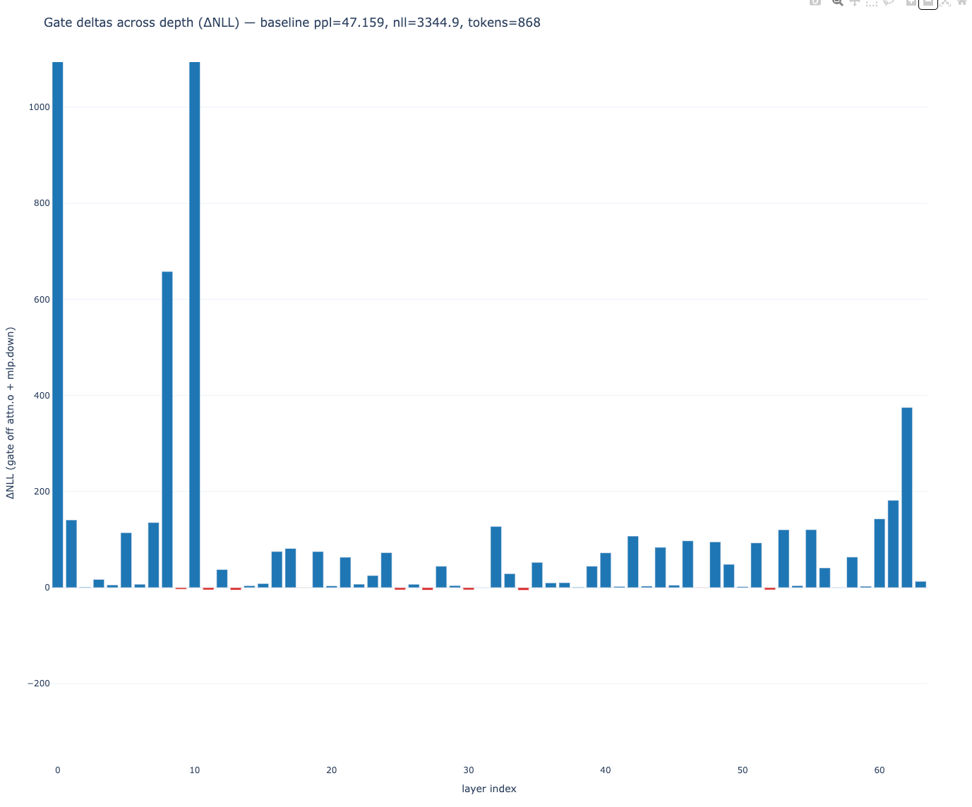
Notes on shapes, and why any of this compiles
q/k/v/o shapes under grouped kv heads trip up most conversions. LLaMA/Qwen keep head_dim constant, so:
If the source had different num_kv_heads than the target, reshape W_k and W_v to [heads, head_dim, in], average or repeat along the head axis to hit the target head count, then fold back. head_dim mismatches are handled by truncate/pad along that axis. For the FFN, keep the out×in rule straight:
Up and gate: [i, h]
Down: [h, i]
The router in an MoE block learned to select a couple experts per token. After averaging, the single dense FFN is an approximation of the expected expert. The concat trick turns into “sum of all experts,” which is not what was trained. That’s why averaging behaved.
Does this generalize to other model families?
It works nicely across the LLaMA ecosystem when the widths match. LLaMA-2, LLaMA-3, Qwen3, and many LLaMA-derivatives share h = 4096 and head_dim = 128 at the 8B scale. KV-heads still differ, so do the GQA remap.
Mixing across different hidden sizes becomes bad. If the weights don’t line up, you’d need adapters between every linear and you quickly build an adapter model, not a splice. ViT-style models or NeoX-style attention have different projections and block ordering, so you’d need bespoke mapping logic.
You can mix instruct and base variants of the same family. Instruction tuning mostly lives in the weights you’re already moving; RoPE and tokenizer must be identical or you get nonsense. If RoPE theta or scaling differs, keep the base config and only transplant blocks. That acts like a “RoPE adapter” because you keep sinusoidal parameters consistent.
The obvious follow-up: can you splice MoE from Mixtral into LLaMA-3-8B? If hidden size and head_dim line up, yes, but the Mixtral MoE FFN layout and gate logits differ. You’d still convert MoE → dense with a family-aware mapping, then interleave. It won’t be cross-family plug-and-play, but it’s doable.
Pushing quality further
A tiny recovery finetune is the best way from here. One pass with low-rank adapters on attention and MLP, BF16, LR around 1e-5, a couple thousand steps on a mixed corpus. That smooths the last few percent of mismatch between transplanted and base blocks. The layer influence scans will flatten out.
Weights surgery can go deeper: per-layer scalar calibration is almost free, and you already saw it works. A soft version is to calibrate q and k per layer so that the mean token RMS matches the base envelope. That’s a deterministic alternative to “try 0.9 and see.”
You can also reverse the interleave ratio. Instead of 36 base + 28 MoE in 64 layers, aim for smaller models like 48 total layers and sample 16 MoE blocks. That gives an 11B-ish composite that’s gentler on memory without blowing up token budgets.
Things to watch out for
RoPE must be consistent across the whole composite. Keep the base config. Tokenizer must match the base. Embeddings should be tied.
Be careful with the very last block. The final projection and the LM head are co-adapted; swapping that block with a different family’s block is a short path to the land of broken losses.
Some blocks don’t look important on small evals. A 900-token probe is fine to find the large ones, but it’s noisy for the small ones. Use a 10k+ token set for the last call.
Wrap-up
You can take a giant MoE model, flatten its experts into dense feed-forwards that match a smaller dense model, interleave those with the base blocks to create a deeper hybrid, and then prove—with simple gates and swaps—that the transplanted blocks carry their weight. The last mile is precision work: replace a weak link or two, trim q/k on the ‘hot’ ones, and leave the tail alone.
My favorite takeaway from all of this is that if hidden size and head_dim line up, you can do a lot of interesting surgery without writing an adapter puddle.
Concatenation does a weird “use all experts all the time” thing and usually fries the block. It did “work” in the sense that tensors saved and loaded, but it pushed the model toward repetitive noise.
Can you provide the source code for the operation?
Source code?